Quantum computing · A visual refresher
Grovers algoritm
Find one marked answer among \(N\) possibilities. Two reflections explain the search; interactive vectors and amplitude columns show how to build it.
This is a refresher on the standard quantum search algorithm. We begin with general \(N\), then use sixteen states for the visual examples. For our spatial implementation, where free evolution supplies the mixing, see Grover implementation with a particle in a Box.
01 / Ordinary Grover
Find one answer among \(N\) possibilities
Imagine \(N\) possible answers, with \(N>1\). Exactly one satisfies a condition, and we can test a proposed answer without already knowing which one will pass. Grover’s algorithm turns this ability to recognize the answer into an efficient way to find it.
Write the candidates as orthonormal basis states \(|j\rangle\), with \(j=0,\ldots,N-1\), and call the unknown marked state \(|w\rangle\). A quantum state assigns an amplitude to each candidate:
A measurement gives \(j\) with probability \(|a_j|^2\). Amplitudes themselves can be negative or complex: their relative phases determine how they interfere. For now, assume we start with an equal, real superposition,
Every candidate initially has probability \(1/N\). We are given an oracle that recognizes the answer by reversing its amplitude’s sign, without measuring the state. We will explain how to prepare \(|s\rangle\) and build the other reflection later. First, what do these two reflections achieve?
In the oracle model, one marked item among \(N\) candidates needs order \(N\) classical queries for a fixed high success probability; Grover needs order \(\sqrt N\). This counts calls to the test. The cost of constructing the oracle and accessing any data still belongs to the physical problem. [Grover, 1996]
02 / The mechanism
Two mirrors make a rotation
A state with \(N\) amplitudes might sound difficult to draw. But the unmarked states all start alike, and these two operations treat them alike. Their amplitudes remain equal. Combine those \(N-1\) states into one normalized direction, perpendicular to the marked direction:
The entire search now fits in the plane spanned by \(|r\rangle\) and \(|w\rangle\). Draw \(|r\rangle\) horizontally and \(|w\rangle\) vertically. A unit arrow represents the state; its vertical coordinate is the marked amplitude, and the square of that coordinate is the success probability. The starting arrow \(|s\rangle\) sits at an angle \(\theta=\arcsin(1/\sqrt N)\) above the horizontal. These are directions in state space, not physical positions.
First mirror: reverse the marked component
The projector \(|w\rangle\langle w|\) extracts the marked component. Subtracting twice that component reverses it while leaving the unmarked component alone. In our plane, the oracle mirrors the arrow across the horizontal \(|r\rangle\) line: an angle \(\alpha\) becomes \(-\alpha\). The marked probability is unchanged.
Second mirror: reflect about the starting direction
This reflection preserves the component parallel to \(|s\rangle\) and reverses the perpendicular component. Its mirror is the tilted \(|s\rangle\) line. Applied after the oracle, it takes the angle \(-\alpha\) to \(2\theta+\alpha\). Together the two mirrors advance the original arrow by \(2\theta\) per round. Starting at \(\theta\), we reach \(3\theta\), then \(5\theta\), then \(7\theta\).
Our visual example: \(N=16\). For the visualizations, we will use sixteen candidates, arranged later on a \(4\times4\) grid. Each starts with probability \(1/16=6.25\%\), and \(\theta\approx14.48^\circ\). The reflection argument above applies to any \(N>1\).
Each click applies one exact reflection. The moving arrow illustrates the geometry between endpoints; it does not depict a gate’s physical time evolution. Continue past three rounds to see the probability fall again.
After \(k\) complete oracle–diffuser pairs, the conventional state and its success probability are
For our sixteen-state example, the first three rounds give 47.27%, 90.84%, and 96.13%. At three rounds the vector is close to the marked axis; a fourth round carries it farther past that axis and drops the probability to 58.17%. The operation is reversible, so it cannot keep pushing probability upward forever. For general \(N\), the first peak is near \(k=\pi/(4\theta)-1/2\); choose a nearby integer number of rounds. Since \(\sin\theta=1/\sqrt N\), the required number of rounds grows as \(\sqrt N\).
The horizontal coordinate belongs to the normalized sum of the \(N-1\) unmarked states, not to one candidate. Each individual unmarked amplitude is that coordinate divided by \(\sqrt{N-1}\). For our sixteen columns, this factor is \(\sqrt{15}\).
03 / Open up the gates
Prepare once. Undo, flip, and return.
We now know what the reflections should do. How can we build them? For \(N=2^n\), an \(n\)-qubit register supplies the basis states, and a Hadamard on every qubit prepares the equal superposition. In our \(N=16\) example, we use four qubits. Initialize them in the known input \(|i\rangle=|0000\rangle\), and apply a Hadamard to each qubit. The single-qubit gate and the whole-register operator are
This supplies the equal starting vector used above. Preparation is performed once, before the repeated search rounds. We also assume a coherent oracle, a known phase flip on \(|i\rangle\), and a final measurement in the computational basis. There are no measurements between gates.
For the oracle, define \(f(j)=1\) for the solution and 0 otherwise. A reversible test \(|j,b\rangle\mapsto|j,b\oplus f(j)\rangle\) becomes a phase oracle when the auxiliary qubit is \(|-\rangle=(|0\rangle-|1\rangle)/\sqrt2\). It leaves that auxiliary state unchanged and kicks a sign onto the tested register: \(O_w|j\rangle=(-1)^{f(j)}|j\rangle\). We can therefore omit the auxiliary qubit from the diagram. Selecting a goal in a demo programs this test; the search algorithm is given the oracle, not the answer’s index.
Build a reflection from a known phase flip
It is easier to reverse one known basis component than to directly address a tilted superposition. Define
- Undo preparation, \(H^\dagger\). Bring the prepared direction \(|s\rangle\) back to the input direction \(|i\rangle\), carrying every component of the current state along with it.
- Flip the initial-state component, \(S_i\). Reverse the amplitude along \(|i\rangle\) and leave every component perpendicular to it unchanged.
- Apply preparation again, \(H\). Carry the reference direction back from \(|i\rangle\) to \(|s\rangle\).
This is the “rotate back, flip, rotate forward” idea. More precisely, we conjugate a simple reflection by the preparation unitary. Undoing preparation sends \(|s\rangle\) to \(|i\rangle\); it does not reset an arbitrary search state to \(|i\rangle\). The intermediate states can leave the two-dimensional search plane, and \(H\) itself need not be a literal rotation within that plane.
In time order the gates are \(H^\dagger\to S_i\to H\). Since \(H^\dagger=H\), the same Hadamard appears on both sides. Matrix multiplication acts from right to left:
The minus sign changes only the global phase. Our reference gate \(S_i\) flips the initial component, so \(M\) flips the prepared direction \(|s\rangle\). This gives \(M=-D\): every output amplitude is the negative of the corresponding output from \(D\). Multiplying the whole state by \(-1\) leaves relative phases and all measurement probabilities unchanged. After \(k\) full rounds, the two conventions differ by \((-1)^k\). The opening vector diagram uses \(D\); the columns retain the signs produced by their gates. [Operator conventions]
Here is the sandwich as simple real-vector geometry. The yellow arrow is the reference \(|s\rangle\); the violet line perpendicular to it is the mirror for our \(M\). Turn the whole picture until the reference lines up with the horizontal initial-state axis, perform the simple reflection, then turn back.
Call the turn \(R\), with \(R|i\rangle=|s\rangle\). The construction is \(RS_iR^{\mathsf T}\): the rightmost operation acts first. This illustrates the same complete reflection as \(HS_iH\). Choose an example vector and watch the reference and mirror travel with it.
- |v0⟩Input vector
- RT1 · Align reference
- Si2 · Reflect
- R3 · Turn back
v = +0.940|i⟩ +0.342|u⟩
Turn the basis → reflect → turn back. Pause or scrub to follow the picture; Previous plays backward. The grey arrow keeps the original vector in the current basis.
How the real picture connects to the Hadamard circuit
For the sixteen-state example, \(|u\rangle\) is the normalized sum of the fifteen states other than \(|i\rangle\), and \(|s\rangle=(|i\rangle+\sqrt{15}|u\rangle)/4\). In this real plane we choose the rotation
Both \(R\) and \(H\) send the initial direction to \(|s\rangle\). Conjugating \(S_i\) with either gives the same complete reflection:
The widget uses \(R\) to make the change of basis visible as a simple turn. Its moving arrows illustrate the geometry between stages. The circuit and column demo retain their actual Hadamard gates.
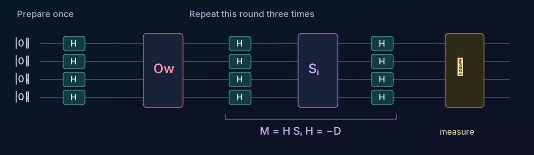
The two Hadamards also mix amplitudes along the way. The column view below lets us follow those intermediate states, gate by gate.
04 / Try the abstract search
Follow the amplitudes, gate by gate
Now separate the vector into its sixteen basis amplitudes. Arrange the states on a \(4\times4\) grid: the first two bits label column x and the last two label row y, so \(j=4x+y\). The lower-left state is our input \(|0000\rangle\); the upper-right state is our example target \(|1111\rangle\). This grid arranges labels; it does not assign a physical distance between states. Column heights show real amplitudes, so a column below zero does not mean negative probability.
For uniform \(|s\rangle\), \(D\) reflects each amplitude about the arithmetic mean \(\mu\). The two operators act as follows:
After the first oracle, fifteen amplitudes are \(+1/4\) and the marked amplitude is \(-1/4\), giving a mean of \(7/32\). Our mixer \(M\) takes them to \(-3/16\) and \(-11/16\), respectively, and the marked probability becomes \((11/16)^2=47.265625\%\). No gate needs to measure the mean: these are fixed linear operators.
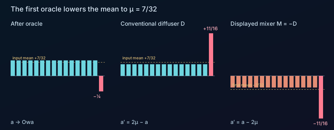
Start with one column. Press Next step to prepare the equal superposition, then apply the oracle. Leave Combine off to see each of the three mixer gates. After the first \(H\) inside that mixer, the input amplitude is \(+7/8\), while the others are \(\pm1/8\). \(S_i\) flips \(+7/8\) to \(-7/8\), and the final \(H\) collects these contributions into the amplified result.
Turn Combine on before entering a mixer to go straight from its input to its output. This uses the same complete operator \(M\), with a direct continuous unitary animation between its endpoints. It does not visit the hidden \(H\text{–}S_i\text{–}H\) checkpoints. During animations the state can be complex; choose the imaginary view to see the part that real column heights leave out.
Loading the column view. The figures and table below also show the exact checkpoint values.
Drag to orbit; scroll or pinch to zoom. The measurement symbol lights at the recommended stop. You can keep stepping.
The yellow mean plane travels with the columns in the combined animation. All real column tips shift by \(-2\mu\), which is \(-7/16\) in the first round, and their mean moves from \(+7/32\) to \(-7/32\). The solid plane shows the current mean; the dashed destination marks its final value.
Why repeating works—and why to stop
Return to the two-dimensional picture at complete round boundaries. Using the same \(|r\rangle\) and \(\theta\) as the opening diagram, the state after \(k\) rounds is
After three rounds we are close to the marked direction. Another round carries us past it. The algorithm is a reversible rotation, so it cannot keep increasing the marked probability forever.
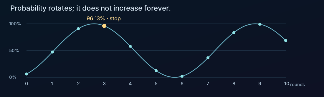
| Checkpoint | Marked \(a_w\) | Each unmarked \(a_j\) | \(P_w\) |
|---|---|---|---|
| Prepared | +0.250000 | +0.250000 | 6.25% |
| Round 1 | −0.687500 | −0.187500 | 47.27% |
| Round 2 | +0.953125 | +0.078125 | 90.84% |
| Round 3 · measure | −0.980469 | +0.050781 | 96.13% |
| Round 4 · overshoot | +0.762695 | −0.166992 | 58.17% |
Even at the recommended stop the unmarked amplitudes need not have the same sign as the marked one. Signs record the full rotation; probability is their squared magnitude. In the full demo, Run full search stops at the first recommended peak. Next step continues beyond it, and Previous step returns to the preceding checkpoint.
What exactly is interpolated in the column animation?
For any Hermitian reflection \(G\text{ with }G^2=I\), the animation uses \(U(p)=(I+G)/2+e^{-i\pi p}(I-G)/2\), for \(0\le p\le1\). At the endpoints it is \(I\) and \(G\), and it preserves the norm throughout. For a real input to a combined mixer, the real heights follow \(a_j(p)=a_j(0)-2\mu\sin^2(\pi p/2)\). Their imaginary parts are \(-\mu\sin(\pi p)\). This is a chosen path for visualizing a discrete gate, not a claim about how every quantum device executes it. The article’s compact viewer uses the Ordinary-Grover branch’s state-vector and 3D rendering code.
The arithmetic-mean formula assumes our input \(|0000\rangle\). Choosing another input in the full demo prepares \(H|i\rangle\) with different signs. The general rule then subtracts \(2s_j\langle s|\psi\rangle\) from each amplitude; the reference guide becomes a set of per-column tiles.
A search carried by a wave
The reflections depend on amplitudes and their phases. What happens when those amplitudes belong to spatial modes of one particle? In Grover implementation with a particle in a Box, we build the search from wave packets, selective phase pulses, and the natural energy spectrum of a square box. The inverse mixing step comes from waiting farther forward in time.
Sources and further reading
The interactive column viewer uses the ordinary Grover implementation from the Grover visualization project.
- Lov K. Grover, A fast quantum mechanical algorithm for database search (1996): the original search algorithm and inversion about the average.
- Gilles Brassard, Peter Høyer, Michele Mosca, and Alain Tapp, Quantum Amplitude Amplification and Estimation (2000): preparation by a general unitary.
- IBM Quantum’s Grover operator documentation: circuit decomposition and the sign convention of the zero-state reflection.
Comments and questions
Share a thought about this post or ask a question.