Quantum computing · Our spatial implementation
Grover implementation with a particle in a Box
One particle, a square box, and a search carried by its wave. The energy spectrum supplies the mixing; a longer forward wait supplies the inverse.
Want a refresher on the search algorithm? Grovers algoritm explains the two reflections and the usual gate construction. Here we focus on our implementation in a particle’s spatial wavefunction.
Free evolution between hard walls can supply Grover’s mixer. We encode the candidates in orthonormal wave packets, let their energy phases evolve, and interrupt the free motion with selective phase pulses. For the sixteen-state example, three search rounds put about 96.13% of the logical probability in the marked mode.
The wave and its probability current make the dynamics visible between gates. Yellow tracer dots sample the density and help us follow its flow; they are a visualization of the evolving wave. Below, we develop the free-box model, add spin, and compare it with a controlled Hadamard mixer. Open the free-box simulation →
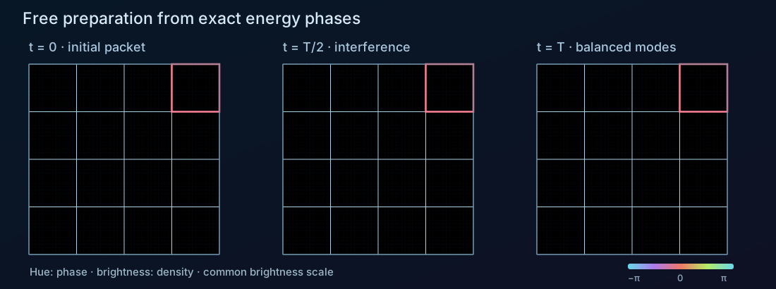
01 / A spatial search register
Give each basis state a wave packet
Our system is one quantum particle confined to a square with hard outer walls. The search candidates are sixteen orthonormal spatial wave packets: four along each axis. They form a sixteen-dimensional state space within one particle’s wavefunction.
Take four sine modes along each axis. On a box of side \(L\), the one-dimensional modes are \(u_n(x)=\sqrt{2/L}\sin(n\pi x/L)\), \(n=1,\ldots,4\). Combine them into four packets \(f_x\), each with its main peak near the center of a different quarter of the interval. Products of two such packets give our \(4\times4\) basis:
The integers \(x,y\) label packets; the capital \(X,Y\) denote continuous physical coordinates. Each coefficient \(c_{xy}\) is the amplitude of one logical search state. Orthonormality makes \(\int|\psi|^2\,\mathrm dX\,\mathrm dY=\sum_{x,y}|c_{xy}|^2\).
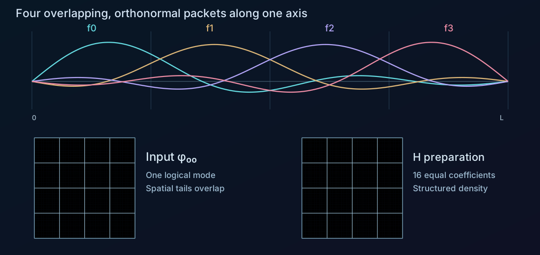
The inner grid lines are labels, not additional walls. The packets overlap in space while remaining orthogonal as functions. Consequently, the probability of the logical outcome \(|x,y\rangle\) is \(|c_{xy}|^2\), whereas the probability of finding the particle inside the corresponding drawn square is the integral of \(|\psi|^2\) over that square. The two readouts are different.
We start in the lower-left packet, \(|i\rangle=|0,0\rangle\). In the illustrated run the target is the upper-right packet, \(|w\rangle=|3,3\rangle\). Choosing that target programs the demo’s phase oracle; the search itself only acts through the oracle.
A measurement that distinguishes the packet modes would read out the logical search result. A simple position measurement reads out position instead. This distinction matters when comparing a grid percentage with the fraction of tracers inside a square.
The precise packet basis
For a \(g\times g\) grid, \(f_j(X)=\sum_{n=1}^{g}T_{jn}u_n(X)\), where \(T_{jn}=\sqrt{2/g}\sin[(j+1/2)n\pi/g]\) for \(n\lt g\), and \(T_{jg}=\sin[(j+1/2)\pi]/\sqrt g\). This real orthogonal transform preserves normalization. The figures use \(g=4\) and \(L=1\). Every packet vanishes at the outer walls; finite sums of sine modes do not have compact support inside one cell.
02 / The box becomes the mixer
Mix by letting the particle evolve
Inside the square, set the potential to zero and keep the hard walls. The Hamiltonian and sine-mode energies are
Here \(n\) and \(\ell\) are positive integer mode numbers and \(m\) is the particle mass. Each sine coefficient simply acquires its own phase, \(b_{n\ell}(t)=e^{-iE_{n\ell}t/\hbar}b_{n\ell}(0)\). The reconstruction in the packet basis can look complicated, but its evolution is known exactly.
For four packets per axis, wait \(T=\pi\hbar/(4E_1)\). The first four one-axis energy phases are \((z,-1,z,1)\), with \(z=e^{-i\pi/4}\). In our packet basis the resulting one-dimensional matrix is
Every entry of \(A\) has magnitude \(1/4\). A localized input therefore evolves into equal logical probabilities, with definite relative phases. The box itself performs balanced preparation and mixing.
Undoing the mixer by waiting forwards
The propagator \(A=U_{\mathrm{box}}(T)\) is not its own inverse. However, the full box spectrum revives at \(T_{\mathrm{rev}}=2\pi\hbar/E_1=8T\). Every mode then returns with exactly its original phase. We can implement \(A^\dagger\) with positive-time free evolution:
The inverse really takes seven times as long as the forward mixer. No time reversal is needed. At 1× playback, \(T\) is 2.4 seconds and the inverse interval is 16.8 seconds.
Assemble the search round
Preparation gives \(|s_A\rangle=A|i\rangle\). We need two selective phase operations: the oracle \(O_w=I-2|w\rangle\langle w|\), which flips the marked mode, and the reference \(S_i=I-2|i\rangle\langle i|\), which flips the known input mode. Undo preparation, apply the reference flip, and prepare again:
A round applies \(O_w\) followed by \(M_A\). In time order: oracle → wait \(7T\) → input phase flip → wait \(T\). Preparation is performed once, before the repeated rounds. This is amplitude amplification about the actual prepared state, even though its coefficients are complex. For the reflection geometry and sign convention, see the refresher’s gate construction. [Amplitude amplification]
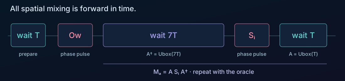
At complete-round boundaries, the marked-mode probability rises from 6.25% to 47.27%, 90.84%, and 96.13%. Stop after three rounds in this example: a fourth drops it to 58.17%. The wave’s intermediate phases and density come from the box dynamics, while the endpoint probabilities follow the usual Grover amplification curve.
Explore the free box → Choose the initial packet and goal directly on the wave, or keep the illustrated defaults. Use Apply next operation to watch preparation and the much longer inverse wait. Keep phase colors on to see the interference that redistributes the wave.
Changing the grid size
The full demo supports \(2\times2\) through \(5\times5\). Write \(g\) for the number of packets per axis, so the scalar search has \(N=g^2\) states. Free preparation uses \(T=T_{\mathrm{rev}}/(2g)\), and its inverse waits \((2g-1)T\). With the box and mass fixed, these two mixing waits always add to one revival period; the phase pulses take additional time.
The query advantage and the encoding’s physical resources are separate questions. Representing \(N\) candidates by \(N\) spatial modes does not by itself provide a scalable replacement for a \(\log_2N\)-qubit device: preparing, controlling, resolving, and measuring those modes also requires resources.
03 / The motion between gates
Follow the probability through the box
During free evolution, the wave determines the scalar Schrödinger probability current. The arrows show this current; yellow tracers are advected with the local transport velocity \(\mathbf v=\mathbf j/\rho\):
The current obeys the continuity equation, \(\partial_t\rho+\nabla\cdot\mathbf j=0\): probability leaves one region by flowing into another. The yellow dots are numerical tracers sampled from \(\rho=|\psi|^2\). Their motion helps us track how that density moves and changes shape. The viewer uses 25,000 small tracers with short trails, so local flow remains readable. The tracer count controls the detail of this visual sampling; the wave, current, and search probabilities are computed independently of it.
The phase pulses need a different transport rule
Free evolution supplies the mixing intervals. The oracle and reference are ideal mode-selective pulses, during which we omit the kinetic Hamiltonian. Each pulse rotates one packet coefficient through half a turn:
Here \(\tau\) is the pulse duration. The logical probabilities stay fixed during a pulse, but spatial density can change because the packets overlap and interfere. A mode projector is therefore not equivalent to applying a local potential inside one drawn square.
For these nonlocal pulses, the scalar demo chooses \(\mathbf j=\nabla\chi\), with \(\nabla^2\chi=-\partial_t\rho\) and zero normal current at the walls. Moving the dots with \(\mathbf v=\mathbf j/\rho\) transports the changing density consistently. This is the curl-free current chosen for the ideal pulse. It satisfies the same continuity equation as the evolving density.
04 / One more degree of freedom
Two amplitudes at every position
We can extend the search by giving the particle spin \(\tfrac12\). Every spatial packet can now carry an up and a down amplitude. Our \(4\times4\) grid encodes 32 joint states \(|x,y,\sigma\rangle\), and the wave becomes a two-component spinor:
Mix position with the same free-box propagator and mix spin with a uniform rotation. With \(R_y(\alpha)=e^{-i\alpha\sigma_y/2}\), where \(\sigma_y\) is the Pauli y matrix, preparation and its inverse are
The spin rotation is an imposed spin-only drive. The spatial motion during mixing is still free; the entire operation also includes this drive. The oracle flips one joint position–spin mode, and \(S_i\) flips the chosen input position–spin mode. The reflection argument is unchanged.
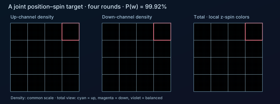
Preparation gives \(1/32\) in every joint mode. The first recommended stop is now four rounds, at approximately 99.9182% marked-mode probability. A position measurement alone does not distinguish up from down. The demo therefore separates joint-mode probabilities from the spatial probability inside the goal box, which includes both spin components.
Spin changes the current, too
Spin introduces an additional contribution to the probability current, which can change the current’s circulation while leaving the density evolution unchanged. The position current used during free evolution with the uniform spin drive includes the convective term and this spin contribution:
In the planar model, the spin term is \((\hbar/2m)(\partial_YM_z,-\partial_XM_z)\), with \(M_z=|\psi_\uparrow|^2-|\psi_\downarrow|^2\). It is divergence-free: it can add circulation and bend the tracer paths without changing the density’s continuity equation. After a selective oracle, position and spin can become entangled. The tracers continue to sample the total density, with both spin components contributing to the current. [Pauli current]
Total · spin colors uses cyan and magenta for opposite local z polarizations. A spinor has no single scalar phase, so that total view has a different legend from the individual up/down phase views. Switch the current arrows between total, transport, and spin current to see which part produces which flow.
How the spin-current tracers are calculated
The simulation displays the planar components of the Pauli probability current. Tracer motion visualizes that current in the two-dimensional density plot. During ideal nonlocal phase pulses it adds a gradient correction \(\nabla u\) satisfying \(\nabla^2u=-\partial_t\rho-\nabla\cdot\mathbf j_{\mathrm P}\), with zero normal derivative at the walls. This retains spin circulation while enforcing continuity. It is a specified extension for these ideal gates, rather than a unique experimental realization of an oracle. The wave coefficients evolve exactly in the retained mode space; tracer advection and sampled current fields have numerical error.
Explore the spin version → Select a joint goal, run four rounds, and compare the spin-resolved result with the total spatial density.
05 / A controlled comparison
Compare with a controlled Hadamard mixer
To separate the spatial encoding from the box’s natural evolution, we also built a controlled model, MultiRegion. It applies \(H=H_1^{\otimes4}\) to the sixteen packet coefficients, where \(H_1\) is the single-qubit Hadamard. The refresher derives this gate construction. Begin with \(\varphi_{00}\), prepare with \(H\), mark \(\varphi_{33}\), then apply \(H^\dagger\), \(S_i\), \(H\). Its gate endpoints reproduce the ordinary four-qubit search in this spatial basis.
To show a continuously moving wave between gates, this model uses an ideal coupling Hamiltonian over a mixing interval of duration \(\tau\). We write it as \(\mathcal H_{\mathrm{mix}}\) to distinguish it from the gate \(H\):
At \(p=1\) this gives \(H\) exactly. The inverse interval follows \(U(-p)\): the endpoint is again \(H\), but the continuous path runs with the opposite coupling. The sine modes give us a spatial basis here; their free kinetic-energy phases are not added during these controlled gates.
The oracle and reference use the mode-selective phase pulses described above. All operations in this comparison model are imposed couplings; free kinetic evolution is omitted.
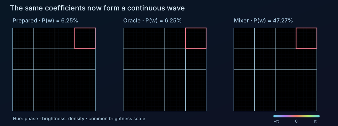
The yellow dots use the gradient-current rule described in the probability-flow section throughout these controlled gates. Comparing this view with the free box reveals how two different continuous dynamics can produce the same marked-mode probabilities at complete rounds.
Controlled mixing on other grids
The \(3\times3\) and \(5\times5\) controlled versions use a balanced Hermitian transform \(B_{(x,y),(u,v)}=e^{2\pi i(xv-yu)/g}/g\), with \(g\) packets per axis, instead of a qubit Hadamard. They amplify 9 or 25 spatial modes.
Explore the controlled wave model → Start with phase colors on. Step through the first oracle and compare the changing density with the unchanged marked-mode percentage.
The experiments
Explore the implementations
Start with the free-box simulation to try the implementation described here. The spin and controlled-wave versions let you compare different dynamics. Ordinary columns accompany the separate refresher and provide a reference for the gate amplitudes.
| Model | States | Preparation | Flow of the dots |
|---|---|---|---|
| Ordinary columns | 16 basis states | \(H=H_1^{\otimes4}\) | Columns show amplitudes; no spatial flow is drawn. |
| Controlled wave | 16 spatial modes | The same \(H\), acting on packet coefficients | A chosen gradient current \(\mathbf j=\nabla\chi\) preserves continuity throughout the controlled gates. |
| Free box | 16 spatial modes | \(A=U_{\mathrm{box}}(T)\) | Schrödinger current during free evolution; chosen gradient transport during phase pulses. |
| Free box + spin | 32 joint position–spin modes | \(U_{\mathrm{box}}(T)\otimes R_y(\pi/2)\) | Planar Pauli current, including spin circulation; a gradient correction enforces continuity during phase pulses. |
Both free-box models still assume ideal mode-selective oracle and reference phase pulses. The spin model also applies a uniform spin drive. The full demos offer other grid sizes.
Choose a simulation to load it here. The wave demos need WebGL2.
Open full free-box demo ↗Choose a view above to start exploring.
Changing the view starts that simulation afresh. Each full demo keeps its own controls and gate implementation. On a small screen, use the full-page link for more room.
Sources and further reading
The packet basis, free-box matrix, numerical figures, and four demos in this article come from the Grover visualization project. The free-box result above follows directly from its sine spectrum and the displayed packet transform. The demos retain their distinct branch dynamics.
- Gilles Brassard, Peter Høyer, Michele Mosca, and Alain Tapp, Quantum Amplitude Amplification and Estimation (2000): preparation by a general unitary A.
- Marek Nowakowski, The Quantum Mechanical Current of the Pauli Equation (1998; published 1999): the spin contribution obtained from the nonrelativistic limit of the Dirac current.
Comments and questions
Share a thought about this post or ask a question.