Educational notebook

Stern-Gerlach in Bohmian Mechanics

What is Spin in Bohmian mechanics?

A spinor wave packet splitting in a Stern-Gerlach magnetic field

Before the magnet

Bohmian mechanics allows us to provide an unusually "detailed" version of what is going on in Stern-Gerlach (SG) experiment. As you may know, in SG we send a spin 1/2- particle (in the original experiment, a silver-atom) through a non-uniform magnetic field. The magnetic field needs to be non-uniform in order couple with the magnetic dipole moment of the particle.

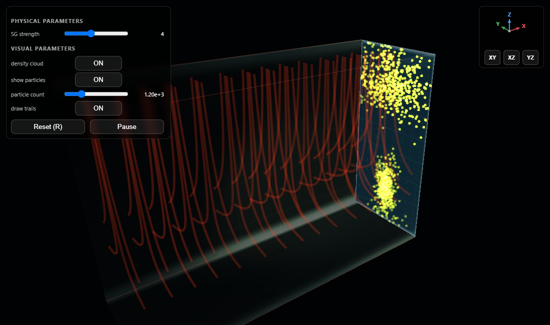
The simulation scene is a tunnel, where the spin half particle travels. You can adjust the spin direction and momentum. The default spin axis is aligned with the motion. Such a state also corresponds to an up/down superposition, as we want it.

The field lines are absent and the packet remains spatially unsplit.

A spin superposition

In bohmian mechanics, the particles do not contain the spin. The spin is in the wave, so to speak. Each Bohmian particle simply follows where the splitting wave happens to guide it.

Let us prepare the spinorial wave function in an equal superposition of \(+z\) and \(-z\) components. The Pauli equation will dictate how the wave components will couple with opposite signs to the magnetic field. This causes the spinor wave to separate into spatially distinct packets.

The wave splits, and the bohmian particles get carried along.

Q: What determines whether a particle ends up in the upper or lower portion of the packet?

A: The position of the particle as the splitting is enacted. If the particle is (roughly) in the upper portion of the packet, the upward wave component will dominate can carry it up. Conversely, if the particle is in the lower portion, it will go along with the downward component of the wave.

In the middle region there is quite a competion for the particles between the packets.

Contextuality of Spin

As we have seen, in Bohmian mechanics the particle does not posses an intrinsic property called spin. The spin is "in the wave". This really is no problem, but may lead to confusion from the point of view of the traditional interpretation.

Let us demonstrate with a simplified version of the SG experiment. This demo allows you to rotate the SG-magnets. Try flipping the SG-apparatus upside down. Now up is down and vise versa, right? Indeed, if you look at the color coding of the wave, you observe that the packet which originally went up, now goes down (and vise versa). Just as one would expect.

However, if you look at the particles, the one that happen to start in the upper portion will still be guided up, and the one starting from the lower portion will be guided down. The particles did not notice the inversion of the field! This is what is referred to as contextuality of spin.

Contextuality is may seem surpricing, even wrong, but only if you hold on to the idea of particles themselves carrying the spin. As soon as you recal the particles just follow the wave, there is nothing mysterious about it whatsoever. And the statistics will remain exactly the same, so empirically the Bohmian mechanics continues to produce the standard predictions of quantum mechanics.

Flip the SG magnet upside down. The spin carrying wave will flip, but the particles will not. Statistics remain the same.

Theory and equations

The Pauli spinor

The "Schrödinger wave" is replaced by a spinorial wave function. Spin-\(\tfrac12\) state has two complex components:

\[ \Psi(\mathbf x,t) = \begin{pmatrix} \psi_+(\mathbf x,t)\\ \psi_-(\mathbf x,t) \end{pmatrix}, \qquad \rho=\Psi^\dagger\Psi . \]

The two components represent amplitudes for opposite spin outcomes along the selected measurement axis.

Magnetic interaction

The Schrödinger wave equation is replaced by the Pauli equation, which contains the coupling between spin and the magnetic field:

\[ i\hbar\frac{\partial\Psi}{\partial t} = \left[ \frac{1}{2m} \left(-i\hbar\nabla-q\mathbf A\right)^2 +q\Phi -\boldsymbol{\mu}\cdot\mathbf B(\mathbf x) \right]\Psi . \]

Here \(q\) is the particle's charge, \(\Phi\) is the scalar potential, and \(\mathbf B=\nabla\times\mathbf A\). A spatial gradient in \(\mathbf B\) gives the two spin components opposite forces and separates their wave packets. The simulation retains the spin-field interaction but neglects the orbital coupling to \(\mathbf A\). For a neutral atom's center of mass, \(q=0\), so this orbital term vanishes while the magnetic-moment coupling remains.

Measurement probabilities

For an initial spin state \(a\lvert +z\rangle+b\lvert -z\rangle\), ideal branch weights are

\[ P(+z)=|a|^2, \qquad P(-z)=|b|^2, \qquad |a|^2+|b|^2=1 . \]

The equal superposition used in the splitting demo has equal Born weights for the two branches.

Bohmian guidance

\[ \mathbf v = \frac{\mathbf j}{\rho}, \qquad \mathbf j = \frac{\hbar}{m}\operatorname{Im} (\Psi^\dagger\nabla\Psi) -\frac{q}{m}\mathbf A\,\rho + \frac{s\hbar}{m} \nabla\times (\Psi^\dagger\boldsymbol{\sigma}\Psi). \]

The particle has one position and one continuous path, guided by the gauge-covariant Pauli current of the full spinor. Equivalently, the vector potential contributes \(-q\mathbf A/m\) directly to \(\mathbf v=\mathbf j/\rho\).

Imagining Physics